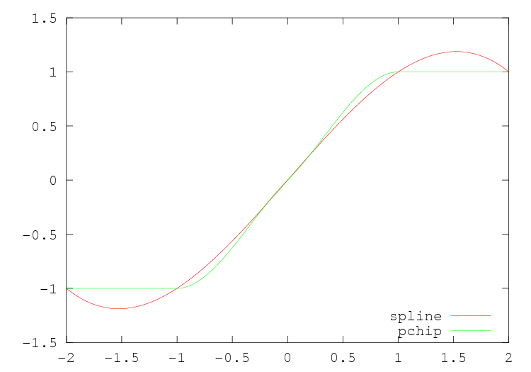
Figure 29.1: Comparison of 'pchip' and 'spline' interpolation methods for a step function
Octave supports several methods for one-dimensional interpolation, most of which are described in this section. Polynomial Interpolation and Interpolation on Scattered Data describe further methods.
One-dimensional interpolation. Interpolate y, defined at the points x, at the points xi. The sample points x must be monotonic. If not specified, x is taken to be the indices of y. If y is an array, treat the columns of y separately.
Method is one of:
- 'nearest'
- Return the nearest neighbor.
- 'linear'
- Linear interpolation from nearest neighbors
- 'pchip'
- Piecewise cubic Hermite interpolating polynomial
- 'cubic'
- Cubic interpolation (same as
pchip)- 'spline'
- Cubic spline interpolation—smooth first and second derivatives throughout the curve
Appending '*' to the start of the above method forces
interp1to assume that x is uniformly spaced, and only x(1)and x(2)are referenced. This is usually faster, and is never slower. The default method is 'linear'.If extrap is the string 'extrap', then extrapolate values beyond the endpoints. If extrap is a number, replace values beyond the endpoints with that number. If extrap is missing, assume NA.
If the string argument 'pp' is specified, then xi should not be supplied and
interp1returns the piecewise polynomial that can later be used withppvalto evaluate the interpolation. There is an equivalence, such thatppval (interp1 (x,y,method, 'pp'),xi) == interp1 (x,y,xi,method, 'extrap').Duplicate points in x specify a discontinuous interpolant. There should be at most 2 consecutive points with the same value. The discontinuous interpolant is right-continuous if x is increasing, left-continuous if it is decreasing. Discontinuities are (currently) only allowed for "nearest" and "linear" methods; in all other cases, x must be strictly monotonic.
An example of the use of
interp1isxf = [0:0.05:10]; yf = sin (2*pi*xf/5); xp = [0:10]; yp = sin (2*pi*xp/5); lin = interp1 (xp, yp, xf); spl = interp1 (xp, yp, xf, "spline"); cub = interp1 (xp, yp, xf, "cubic"); near = interp1 (xp, yp, xf, "nearest"); plot (xf, yf, "r", xf, lin, "g", xf, spl, "b", xf, cub, "c", xf, near, "m", xp, yp, "r*"); legend ("original", "linear", "spline", "cubic", "nearest")See also: interpft.
There are some important differences between the various interpolation methods. The 'spline' method enforces that both the first and second derivatives of the interpolated values have a continuous derivative, whereas the other methods do not. This means that the results of the 'spline' method are generally smoother. If the function to be interpolated is in fact smooth, then 'spline' will give excellent results. However, if the function to be evaluated is in some manner discontinuous, then 'pchip' interpolation might give better results.
This can be demonstrated by the code
     t = -2:2;
     dt = 1;
     ti =-2:0.025:2;
     dti = 0.025;
     y = sign(t);
     ys = interp1(t,y,ti,'spline');
     yp = interp1(t,y,ti,'pchip');
     ddys = diff(diff(ys)./dti)./dti;
     ddyp = diff(diff(yp)./dti)./dti;
     figure(1);
     plot (ti, ys,'r-', ti, yp,'g-');
     legend('spline','pchip',4);
     figure(2);
     plot (ti, ddys,'r+', ti, ddyp,'g*');
     legend('spline','pchip');
The result of which can be seen in fig:interpderiv1 and fig:interpderiv2.
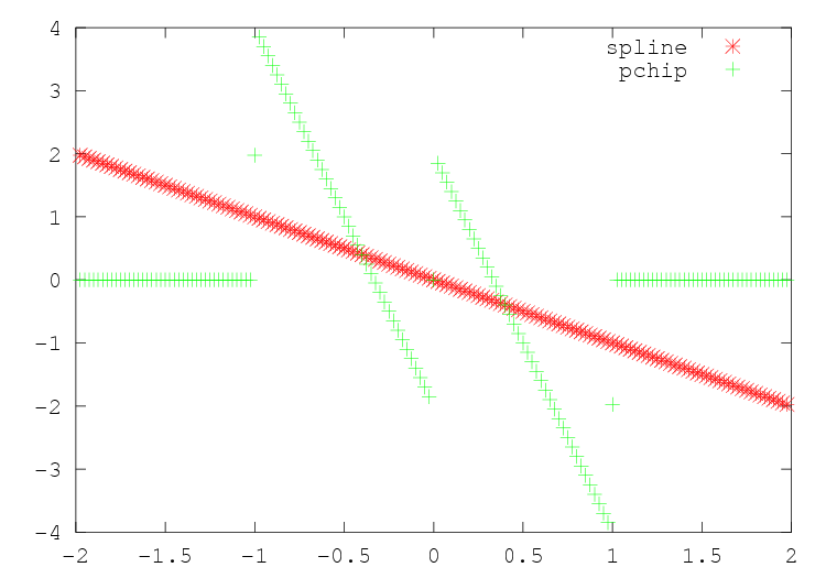
Figure 29.2: Comparison of the second derivative of the 'pchip' and 'spline' interpolation methods for a step function
A simplified version of interp1 that performs only linear
interpolation is available in interp1q. This argument is slightly
faster than interp1 as to performs little error checking.
One-dimensional linear interpolation without error checking. Interpolates y, defined at the points x, at the points xi. The sample points x must be a strictly monotonically increasing column vector. If y is an array, treat the columns of y separately. If y is a vector, it must be a column vector of the same length as x.
Values of xi beyond the endpoints of the interpolation result in NA being returned.
Note that the error checking is only a significant portion of the execution time of this
interp1if the size of the input arguments is relatively small. Therefore, the benefit of usinginterp1qis relatively small.See also: interp1.
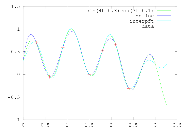
Fourier interpolation, is a resampling technique where a signal is converted to the frequency domain, padded with zeros and then reconverted to the time domain.
Fourier interpolation. If x is a vector, then x is resampled with n points. The data in x is assumed to be equispaced. If x is an array, then operate along each column of the array separately. If dim is specified, then interpolate along the dimension dim.
interpftassumes that the interpolated function is periodic, and so assumptions are made about the end points of the interpolation.See also: interp1.
There are two significant limitations on Fourier interpolation. Firstly,
the function signal is assumed to be periodic, and so non-periodic
signals will be poorly represented at the edges. Secondly, both the
signal and its interpolation are required to be sampled at equispaced
points. An example of the use of interpft is
     t = 0 : 0.3 : pi; dt = t(2)-t(1);
     n = length (t); k = 100;
     ti = t(1) + [0 : k-1]*dt*n/k;
     y = sin (4*t + 0.3) .* cos (3*t - 0.1);
     yp = sin (4*ti + 0.3) .* cos (3*ti - 0.1);
     plot (ti, yp, 'g', ti, interp1(t, y, ti, 'spline'), 'b', ...
           ti, interpft (y, k), 'c', t, y, 'r+');
     legend ('sin(4t+0.3)cos(3t-0.1','spline','interpft','data');
which demonstrates the poor behavior of Fourier interpolation for non-periodic functions, as can be seen in fig:interpft.
In additional the support function spline and lookup that
underlie the interp1 function can be called directly.
Finding Elements and Checking Conditions
Return the cubic spline interpolant of points x and y.
When called with two arguments, return the piecewise polynomial pp that may be used with
ppvalto evaluate the polynomial at specific points. When called with a third input argument,splineevaluates the spline at the points xi. The third calling formspline (x,y,xi)is equivalent toppval (spline (x,y),xi).The variable x must be a vector of length n. y can be either a vector or array. If y is a vector it must have a length of either n or n
+ 2. If the length of y is n, then the "not-a-knot" end condition is used. If the length of y is n+ 2, then the first and last values of the vector y are the values of the first derivative of the cubic spline at the endpoints.If y is an array, then the size of y must have the form
[s1,s2, ...,sk,n]or[s1,s2, ...,sk,n+ 2]. The array is reshaped internally to a matrix where the leading dimension is given by s1*s2* ... *sk and each row of this matrix is then treated separately. Note that this is exactly opposite tointerp1but is done for matlab compatibility.